1.13. Dislib tutorial
This tutorial will show the basics of using dislib.
Setup
First, we need to start an interactive PyCOMPSs session:
[1]:
import os
os.environ["ComputingUnits"] = "1"

import pycompss.interactive as ipycompss
if 'BINDER_SERVICE_HOST' in os.environ:
    ipycompss.start(graph=True,
                    project_xml='../xml/project.xml',
                    resources_xml='../xml/resources.xml')
else:
    ipycompss.start(graph=True, monitor=1000)
********************************************************
**************** PyCOMPSs Interactive ******************
********************************************************
*          .-~~-.--.           ______         ___      *
*         :         )         |____  \       /   |     *
*   .~ ~ -.\       /.- ~~ .      __) |      /_/| |     *
*   >       `.   .'       <     |__  |         | |     *
*  (         .- -.         )   ____) |   _     | |     *
*   `- -.-~  `- -'  ~-.- -'   |______/  |_|    |_|     *
*     (        :        )           _ _ .-:            *
*      ~--.    :    .--~        .-~  .-~  }            *
*          ~-.-^-.-~ \_      .~  .-~   .~              *
*                   \ \ '     \ '_ _ -~                *
*                    \`.\`.    //                      *
*           . - ~ ~-.__\`.\`-.//                       *
*       .-~   . - ~  }~ ~ ~-.~-.                       *
*     .' .-~      .-~       :/~-.~-./:                 *
*    /_~_ _ . - ~                 ~-.~-._              *
*                                     ~-.<             *
********************************************************
* - Starting COMPSs runtime...                         *
* - Log path : /home/user/.COMPSs/Interactive_13/
* - PyCOMPSs Runtime started... Have fun!              *
********************************************************
Next, we import dislib and we are all set to start working!
[2]:
import dislib as ds
Distributed arrays
The main data structure in dislib is the distributed array (or ds-array). These arrays are a distributed representation of a 2-dimensional array that can be operated as a regular Python object. Usually, rows in the array represent samples, while columns represent features.
To create a random array we can run the following NumPy-like command:
[3]:
x = ds.random_array(shape=(500, 500), block_size=(100, 100))
print(x.shape)
x
(500, 500)
[3]:
ds-array(blocks=(...), top_left_shape=(100, 100), reg_shape=(100, 100), shape=(500, 500), sparse=False)
Now x is a 500x500 ds-array of random numbers stored in blocks of 100x100 elements. Note that x is not stored in memory. Instead, random_array generates the contents of the array in tasks that are usually executed remotely. This allows the creation of really big arrays.
The content of x is a list of Futures that represent the actual data (wherever it is stored).
To see this, we can access the _blocks field of x:
[4]:
x._blocks[0][0]
[4]:
<pycompss.runtime.management.classes.Future at 0x7f0428791240>
block_size is useful to control the granularity of dislib algorithms.
To retrieve the actual contents of x, we use collect, which synchronizes the data and returns the equivalent NumPy array:
[5]:
x.collect()
[5]:
array([[0.48604732, 0.68571232, 0.98557605, ..., 0.51530027, 0.39511585,
        0.42942001],
       [0.03398195, 0.40964073, 0.5437061 , ..., 0.16162333, 0.79046618,
        0.71677277],
       [0.82399233, 0.80869154, 0.16965568, ..., 0.79380114, 0.31004525,
        0.51511589],
       ...,
       [0.57630698, 0.72028925, 0.11842501, ..., 0.92236462, 0.5837854 ,
        0.92114111],
       [0.84521256, 0.17909749, 0.42140394, ..., 0.95331429, 0.01587735,
        0.58532187],
       [0.81065273, 0.5666422 , 0.65635218, ..., 0.58820423, 0.42493203,
        0.84351429]])
Another way of creating ds-arrays is using array-like structures like NumPy arrays or lists:
[6]:
x1 = ds.array([[1, 2, 3], [4, 5, 6]], block_size=(1, 3))
x1
[6]:
ds-array(blocks=(...), top_left_shape=(1, 3), reg_shape=(1, 3), shape=(2, 3), sparse=False)
Distributed arrays can also store sparse data in CSR format:
[7]:
from scipy.sparse import csr_matrix

sp = csr_matrix([[0, 0, 1], [1, 0, 1]])
x_sp = ds.array(sp, block_size=(1, 3))
x_sp
[7]:
ds-array(blocks=(...), top_left_shape=(1, 3), reg_shape=(1, 3), shape=(2, 3), sparse=True)
In this case, collect returns a CSR matrix as well:
[8]:
x_sp.collect()
[8]:
<2x3 sparse matrix of type '<class 'numpy.int64'>'
        with 3 stored elements in Compressed Sparse Row format>
Loading data
A typical way of creating ds-arrays is to load data from disk. Dislib currently supports reading data in CSV and SVMLight formats like this:
[9]:
x, y = ds.load_svmlight_file("./files/libsvm/1", block_size=(20, 100), n_features=780, store_sparse=True)

print(x)

csv = ds.load_txt_file("./files/csv/1", block_size=(500, 122))

print(csv)
ds-array(blocks=(...), top_left_shape=(20, 100), reg_shape=(20, 100), shape=(61, 780), sparse=True)
ds-array(blocks=(...), top_left_shape=(500, 122), reg_shape=(500, 122), shape=(4235, 122), sparse=False)
Slicing
Similar to NumPy, ds-arrays support the following types of slicing:
(Note that slicing a ds-array creates a new ds-array)
[10]:
x = ds.random_array((50, 50), (10, 10))
Get a single row:
[11]:
x[4]
[11]:
ds-array(blocks=(...), top_left_shape=(1, 10), reg_shape=(10, 10), shape=(1, 50), sparse=False)
Get a single element:
[12]:
x[2, 3]
[12]:
ds-array(blocks=(...), top_left_shape=(1, 1), reg_shape=(1, 1), shape=(1, 1), sparse=False)
Get a set of rows or a set of columns:
[13]:
# Consecutive rows
print(x[10:20])

# Consecutive columns
print(x[:, 10:20])

# Non consecutive rows
print(x[[3, 7, 22]])

# Non consecutive columns
print(x[:, [5, 9, 48]])
ds-array(blocks=(...), top_left_shape=(10, 10), reg_shape=(10, 10), shape=(10, 50), sparse=False)
ds-array(blocks=(...), top_left_shape=(10, 10), reg_shape=(10, 10), shape=(50, 10), sparse=False)
ds-array(blocks=(...), top_left_shape=(3, 10), reg_shape=(10, 10), shape=(3, 50), sparse=False)
ds-array(blocks=(...), top_left_shape=(10, 3), reg_shape=(10, 10), shape=(50, 3), sparse=False)
Get any set of elements:
[14]:
x[0:5, 40:45]
[14]:
ds-array(blocks=(...), top_left_shape=(5, 5), reg_shape=(10, 10), shape=(5, 5), sparse=False)
Other functions
Apart from this, ds-arrays also provide other useful operations like transpose and mean:
[15]:
x.mean(axis=0).collect()
[15]:
array([0.51352356, 0.49396794, 0.4661033 , 0.48026991, 0.50136143,
       0.49323405, 0.51248831, 0.51658519, 0.4904544 , 0.47166468,
       0.50245676, 0.49936659, 0.47499634, 0.52566765, 0.53676456,
       0.59127036, 0.50947458, 0.47320677, 0.42695456, 0.54335201,
       0.51780756, 0.49855486, 0.53845333, 0.37299501, 0.51229418,
       0.43110043, 0.47262688, 0.41698864, 0.54994596, 0.46676007,
       0.46070067, 0.48861301, 0.45868291, 0.53380687, 0.50555055,
       0.53453463, 0.43711111, 0.52115681, 0.48152436, 0.49215593,
       0.41552034, 0.47669533, 0.5610678 , 0.43511911, 0.49611885,
       0.44116871, 0.42241364, 0.48626255, 0.51636529, 0.44251849])
[16]:
x.transpose().collect()
[16]:
array([[0.02733543, 0.65891797, 0.36654465, ..., 0.52109164, 0.86395718,
        0.93593907],
       [0.41462264, 0.97419918, 0.14124931, ..., 0.15893453, 0.49486474,
        0.14138483],
       [0.91312707, 0.53860404, 0.96686988, ..., 0.78763956, 0.18268972,
        0.20551984],
       ...,
       [0.19468602, 0.62184611, 0.81007025, ..., 0.88719987, 0.55132466,
        0.32694948],
       [0.19221646, 0.64678511, 0.98416872, ..., 0.18736269, 0.51392039,
        0.59614856],
       [0.49591758, 0.17913008, 0.11419029, ..., 0.02701779, 0.22316829,
        0.78426262]])
Machine learning with dislib
Dislib provides an estimator-based API very similar to scikit-learn. To run an algorithm, we first create an estimator. For example, a K-means estimator:
[17]:
from dislib.cluster import KMeans

km = KMeans(n_clusters=3)
Now, we create a ds-array with some blob data, and fit the estimator:
[18]:
from sklearn.datasets import make_blobs

# create ds-array
x, y = make_blobs(n_samples=1500)
x_ds = ds.array(x, block_size=(500, 2))

km.fit(x_ds)
[18]:
KMeans(n_clusters=3, random_state=RandomState(MT19937) at 0x7F040C5D6440)
Finally, we can make predictions on new (or the same) data:
[19]:
y_pred = km.predict(x_ds)
y_pred
[19]:
ds-array(blocks=(...), top_left_shape=(500, 1), reg_shape=(500, 1), shape=(1500, 1), sparse=False)
y_pred is a ds-array of predicted labels for x_ds
Let’s plot the results
[20]:
%matplotlib inline
import matplotlib.pyplot as plt


centers = km.centers

# set the color of each sample to the predicted label
plt.scatter(x[:, 0], x[:, 1], c=y_pred.collect())

# plot the computed centers in red
plt.scatter(centers[:, 0], centers[:, 1], c='red')
[20]:
<matplotlib.collections.PathCollection at 0x7f03cb313e80>
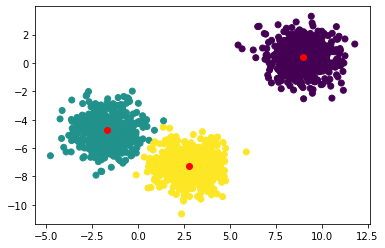
Note that we need to call y_pred.collect() to retrieve the actual labels and plot them. The rest is the same as if we were using scikit-learn.
Now let’s try a more complex example that uses some preprocessing tools.
First, we load a classification data set from scikit-learn into ds-arrays.
Note that this step is only necessary for demonstration purposes. Ideally, your data should be already loaded in ds-arrays.
[21]:
from sklearn.datasets import load_breast_cancer
from sklearn.model_selection import train_test_split

x, y = load_breast_cancer(return_X_y=True)

x_train, x_test, y_train, y_test = train_test_split(x, y)

x_train = ds.array(x_train, block_size=(100, 10))
y_train = ds.array(y_train.reshape(-1, 1), block_size=(100, 1))

x_test = ds.array(x_test, block_size=(100, 10))
y_test = ds.array(y_test.reshape(-1, 1), block_size=(100, 1))
Next, we can see how support vector machines perform in classifying the data. We first fit the model (ignore any warnings in this step):
[22]:
from dislib.classification import CascadeSVM

csvm = CascadeSVM()

csvm.fit(x_train, y_train)
/home/user/github/dislib/dislib/classification/csvm/base.py:395: RuntimeWarning: overflow encountered in exp
  k = np.exp(k)
/home/user/github/dislib/dislib/classification/csvm/base.py:363: RuntimeWarning: invalid value encountered in double_scalars
  delta = np.abs((w - self._last_w) / self._last_w)
[22]:
CascadeSVM()
and now we can make predictions on new data using csvm.predict(), or we can get the model accuracy on the test set with:
[23]:
score = csvm.score(x_test, y_test)
score represents the classifier accuracy, however, it is returned as a Future. We need to synchronize to get the actual value:
[24]:
from pycompss.api.api import compss_wait_on

print(compss_wait_on(score))
0.6503496503496503
The accuracy should be around 0.6, which is not very good. We can scale the data before classification to improve accuracy. This can be achieved using dislib’s StandardScaler.
The StandardScaler provides the same API as other estimators. In this case, however, instead of making predictions on new data, we transform it:
[25]:
from dislib.preprocessing import StandardScaler

sc = StandardScaler()

# fit the scaler with train data and transform it
scaled_train = sc.fit_transform(x_train)

# transform test data
scaled_test = sc.transform(x_test)
Now scaled_train and scaled_test are the scaled samples. Let’s see how SVM perfroms now.
[26]:
csvm.fit(scaled_train, y_train)
score = csvm.score(scaled_test, y_test)
print(compss_wait_on(score))
0.993006993006993
The new accuracy should be around 0.9, which is a great improvement!
Close the session
To finish the session, we need to stop PyCOMPSs:
[27]:
ipycompss.stop()
********************************************************
*************** STOPPING PyCOMPSs ******************
********************************************************
Checking if any issue happened.
Warning: some of the variables used with PyCOMPSs may
         have not been brought to the master.
********************************************************