Welcome to the guide for getting started with COMPSs!
This section will walk you through the simple process of installing the
COMPSs framework and creating your very first application.
Following these steps, you will be able to quickly set up your environment,
understand the basic structure of a COMPSs application, and see a working
application in action.
Let’s dive in and get started!
Install COMPSs
Warning
For macOS distributions, only installations local to the user are supported (both with pip and building
from sources). This is due to the System Integrity Protection (SIP) implemented in the newest versions of
macOS, that does not allow modifications in the /System directory, even when having root permissions in the
machine.
Warning
There is no support for Windows, but COMPSs can be installed and used in Windows by using WSL.
Choose the installation method:
Requirements:
Ensure that the required system Dependencies are installed.
Check that your JAVA_HOME environment variable points to the Java JDK folder, that the GRADLE_HOME environment variable points to the GRADLE folder, and the gradle binary is in the PATH environment variable.
COMPSs will be installed within the $HOME/.local/ folder (or alternatively within the active virtual environment).
$ pipinstallpycompss-v
Important
Please, update the environment after installing COMPSs:
$ source~/.bashrc# or alternatively reboot the machine
If installed within a virtual environment, deactivate and activate
it to ensure that the environment is properly updated.
Warning
If using Ubuntu 18.04 or higher, you will need to comment
some lines of your .bashrc and do a complete logout.
Please, check the Post installation
Section for detailed instructions.
Ensure that the required system Dependencies are installed.
Check that your JAVA_HOME environment variable points to the Java JDK folder, that the GRADLE_HOME environment variable points to the GRADLE folder, and the gradle binary is in the PATH environment variable.
COMPSs will be installed within the /usr/lib64/pythonX.Y/site-packages/pycompss/ folder.
$ sudo-Epipinstallpycompss-v
Important
Please, update the environment after installing COMPSs:
$ source/etc/profile.d/compss.sh# or alternatively reboot the machine
Warning
If using Ubuntu 18.04 or higher, you will need to comment
some lines of your .bashrc and do a complete logout.
Please, check the Post installation
Section for detailed instructions.
Ensure that the required system Dependencies are installed.
Check that your JAVA_HOME environment variable points to the Java JDK folder, that the GRADLE_HOME environment variable points to the GRADLE folder, and the gradle binary is in the PATH environment variable.
Ensure that the required system Dependencies are installed.
Check that your JAVA_HOME environment variable points to the Java JDK folder, that the GRADLE_HOME environment variable points to the GRADLE folder, and the gradle binary is in the PATH environment variable.
Since the PyCOMPSs CLI package is available in PyPI (pycompss-cli), it can be easily installed with pip as follows:
$ python3-mpipinstallpycompss-cli
A complete guide about the PyCOMPSs CLI installation and usage can be found in the 🪄 CLI Section.
Tip
Please, check the PyCOMPSs CLI Installation Section for the further information with regard to the requirements installation and troubleshooting.
Write your first app
Choose your flavour:
Application Overview
A COMPSs application is composed of three parts:
Main application code: the code that is executed sequentially and
contains the calls to the user-selected methods that will be executed
by the COMPSs runtime as asynchronous parallel tasks.
Remote methods code: the implementation of the tasks.
Task definition interface: It is a Java annotated interface which
declares the methods to be run as remote tasks along with metadata
information needed by the runtime to properly schedule the tasks.
The main application file name has to be the same of the main class and
starts with capital letter, in this case it is Simple.java. The Java
annotated interface filename is application name + Itf.java, in this
case it is SimpleItf.java. And the code that implements the remote
tasks is defined in the application name + Impl.java file, in this
case it is SimpleImpl.java.
All code examples are in the /home/compss/tutorial_apps/java/ folder
of the development environment.
Main application code
In COMPSs, the user’s application code is kept unchanged, no API calls
need to be included in the main application code in order to run the
selected tasks on the nodes.
The COMPSs runtime is in charge of replacing the invocations to the
user-selected methods with the creation of remote tasks also taking care
of the access to files where required. Let’s consider the Simple
application example that takes an integer as input parameter and
increases it by one unit.
The main application code of Simple application is shown in the following
code block. It is executed sequentially until the call to the increment()
method. COMPSs, as mentioned above, replaces the call to this method with
the generation of a remote task that will be executed on an available node.
Code 1 Simple in Java (Simple.java)
packagesimple;importjava.io.FileInputStream;importjava.io.FileOutputStream;importjava.io.IOException;importsimple.SimpleImpl;publicclassSimple{publicstaticvoidmain(String[]args){StringcounterName="counter";intinitialValue=args[0];//--------------------------------------------------------------//// Creation of the file which will contain the counter variable ////--------------------------------------------------------------//try{FileOutputStreamfos=newFileOutputStream(counterName);fos.write(initialValue);System.out.println("Initial counter value is "+initialValue);fos.close();}catch(IOExceptionioe){ioe.printStackTrace();}//----------------------------------------------//// Execution of the program ////----------------------------------------------//SimpleImpl.increment(counterName);//----------------------------------------------//// Reading from an object stored in a File ////----------------------------------------------//try{FileInputStreamfis=newFileInputStream(counterName);System.out.println("Final counter value is "+fis.read());fis.close();}catch(IOExceptionioe){ioe.printStackTrace();}}}
Remote methods code
The following code contains the implementation of the remote method of
the Simple application that will be executed remotely by COMPSs.
This Java interface is used to declare the methods to be executed
remotely along with Java annotations that specify the necessary metadata
about the tasks. The metadata can be of three different types:
For each parameter of a method, the data type (currently File type,
primitive types and the String type are supported) and its
directions (IN, OUT, INOUT, COMMUTATIVE or CONCURRENT).
The Java class that contains the code of the method.
The constraints that a given resource must fulfill to execute the
method, such as the number of processors or main memory size.
The task description interface of the Simple app example is shown in the
following figure. It includes the description of the Increment() method
metadata. The method interface contains a single input parameter, a string
containing a path to the file counterFile. In this example there are
constraints on the minimum number of processors and minimum memory size
needed to run the method.
Code 3 Interface of the Simple application (SimpleItf.java)
A COMPSs Java application needs to be packaged in a jar file
containing the class files of the main code, of the methods
implementations and of the Itf annotation. This jar package can be
generated using the commands available in the Java SDK or creating your
application as a Apache Maven project.
To integrate COMPSs in the maven compile process you just need to add the
compss-api artifact as dependency in the application project.
In order to properly compile the code, the CLASSPATH variable has to
contain the path of the compss-engine.jar package. The default COMPSs
installation automatically add this package to the CLASSPATH; please
check that your environment variable CLASSPATH contains the
compss-engine.jar location by running the following command:
$ echo$CLASSPATH|grepcompss-engine
If the result of the previous command is empty it means that you are
missing the compss-engine.jar package in your CLASSPATH. We recommend
to automatically load the variable by editing the .bashrc file:
$ echo"# COMPSs variables for Java compilation">>~/.bashrc
$ echo"export CLASSPATH=$CLASSPATH:/opt/COMPSs/Runtime/compss-engine.jar">>~/.bashrc
Application execution
A Java COMPSs application is executed through the runcompss script. An
example of an invocation of the script is:
In addition to Java, COMPSs supports the execution of applications
written in other languages by means of bindings. A binding manages the
interaction of the no-Java application with the COMPSs Java runtime,
providing the necessary language translation.
Let’s write your first Python application parallelized with PyCOMPSs.
Consider the following code:
Code 4 increment.py
importtimefrompycompss.api.apiimportcompss_wait_onfrompycompss.api.taskimporttask@task(returns=1)defincrement(value):time.sleep(value*2)# mimic some computational timereturnvalue+1defmain():values=[1,2,3,4]start_time=time.time()forposinrange(len(values)):values[pos]=increment(values[pos])values=compss_wait_on(values)assertvalues==[2,3,4,5]print(values)print("Elapsed time: "+str(time.time()-start_time))if__name__=='__main__':main()
This code increments the elements of an array (values) by calling
iteratively to the increment function.
The increment function sleeps the number of seconds indicated by the
value parameter to represent some computational time.
On a normal python execution, each element of the array will be
incremented after the other (sequentially), accumulating the
computational time.
PyCOMPSs is able to parallelize this loop thanks to its @task
decorator, and synchronize the results with the compss_wait_on
API call.
Note
If you are using the PyCOMPSs CLI (pycompss-cli),
it is time to deploy the COMPSs environment within your current folder:
$ pycompssinit
Please, be aware that the first time needs to download the docker image from the
repository, and it may take a while.
Copy and paste the increment code it intoincrement.py.
Execution
Now let’s execute increment.py. To this end, we will use the
runcompss script provided by COMPSs:
$ runcompss-gincrement.py
[Output in next step]
Or alternatively, the pycompssrun command if using the PyCOMPSs CLI
(which wraps the runcompss command and launches it within the COMPSs’ docker
container):
$ pycompssrun-gincrement.py
[Output in next step]
Note
The -g flag enables the task dependency graph generation (used later).
The runcompss command has a lot of supported options that can be checked with the -h flag.
They can also be used within the pycompssrun command.
Tip
It is possible to run also with the python command using the pycompss module,
which accepts the same flags as runcompss:
$ python-mpycompss-gincrement.py# Parallel execution [Output in next step]
Having PyCOMPSs installed also enables to run the same code sequentially without the need of removing the PyCOMPSs syntax.
$ runcompss-gincrement.py
[ INFO] Inferred PYTHON language [ INFO] Using default location for project file: /opt/COMPSs/Runtime/configuration/xml/projects/default_project.xml [ INFO] Using default location for resources file: /opt/COMPSs/Runtime/configuration/xml/resources/default_resources.xml [ INFO] Using default execution type: compss ----------------- Executing increment.py -------------------------- WARNING: COMPSs Properties file is null. Setting default values [(433) API] - Starting COMPSs Runtime v3.4 [2, 3, 4, 5] Elapsed time: 11.5068922043 [(4389) API] - Execution Finished ------------------------------------------------------------
Nice! it run successfully in my 8 core laptop, we have the expected output,
and PyCOMPSs has been able to run the increment.py application in almost half
of the time required by the sequential execution. What happened under the hood?
COMPSs started a master and one worker (by default configured to execute up to four tasks at the same time)
and executed the application (offloading the tasks execution to the worker).
Let’s check the task dependency graph to see the parallelism that
COMPSs has extracted and taken advantage of.
Task dependency graph
COMPSs stores the generated task dependency graph within the
$HOME/.COMPSs/<APP_NAME>_<00-99>/monitor directory in dot format.
The generated graph is complete_graph.dot file, which can be
displayed with any dot viewer.
Tip
COMPSs provides the compss_gengraph script which converts the
given dot file into pdf.
$ cd$HOME/.COMPSs/increment.py_01/monitor
$ compss_gengraphcomplete_graph.dot
$ evincecomplete_graph.pdf# or use any other pdf viewer you like
It is also available within the PyCOMPSs CLI:
$ cd$HOME/.COMPSs/increment.py_01/monitor
$ pycompssgengraphcomplete_graph.dot
$ evincecomplete_graph.pdf# or use any other pdf viewer you like
And you should see:
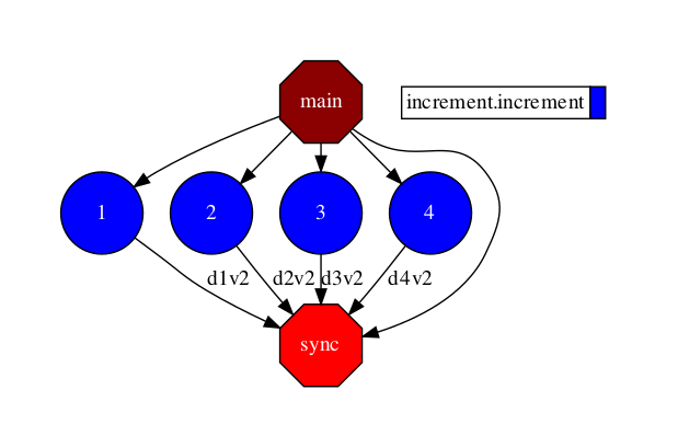
Figure 1 The dependency graph of the increment application
COMPSs has detected that the increment of each element is independent,
and consequently, that all of them can be done in parallel. In this
particular application, there are four increment tasks, and since
the worker is able to run four tasks at the same time, all of them can
be executed in parallel saving precious time.
Check the performance
Let’s run it again with the tracing flag enabled:
$ runcompss-tincrement.py
[ INFO] Inferred PYTHON language [ INFO] Using default location for project file: /opt/COMPSs//Runtime/configuration/xml/projects/default_project.xml [ INFO] Using default location for resources file: /opt/COMPSs//Runtime/configuration/xml/resources/default_resources.xml [ INFO] Using default execution type: compss ----------------- Executing increment.py -------------------------- Welcome to Extrae 3.5.3 [... Extrae prolog ...] WARNING: COMPSs Properties file is null. Setting default values [(434) API] - Starting COMPSs Runtime v3.4 [2, 3, 4, 5] Elapsed time: 13.1016821861 [... Extrae eplilog ...] mpi2prv: Congratulations! ./trace/increment.py_compss_trace_1587562240.prv has been generated. [(24117) API] - Execution Finished ------------------------------------------------------------
The execution has finished successfully and the trace has been generated
in the $HOME/.COMPSs/<APP_NAME>_<00-99>/trace directory in prv format,
which can be displayed and analyzed with PARAVER.
Once Paraver has started, lets visualize the tasks:
Click in File and then in LoadConfiguration
Look for /PATH/TO/COMPSs/Dependencies/paraver/cfgs/compss_tasks.cfg and click Open.
Note
In the case of using the PyCOMPSs CLI, the configuration files can be
obtained by downloading them from the COMPSs repositoy.
And you should see:
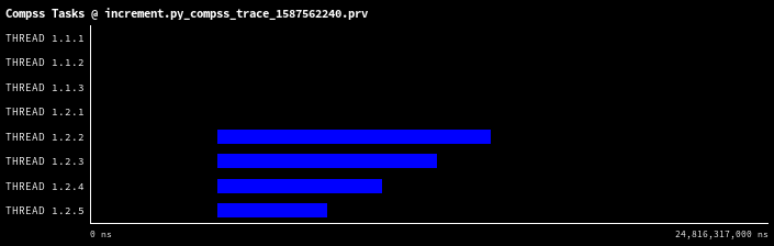
Figure 2 Trace of the increment application
The X axis represents the time, and the Y axis the deployed processes
(the first three (1.1.1-1.1.3) belong to the master and the fourth belongs
to the master process in the worker (1.2.1) whose events are
shown with the compss_runtime.cfg configuration file).
The increment tasks are depicted in blue.
We can quickly see that the four increment tasks have been executed in parallel
(one per core), and that their lengths are different (depending on the
computing time of the task represented by the time.sleep(value*2) line).
Paraver is a very powerful tool for performance analysis. For more information,
check the 🎯 Tracing Section.
Note
If you are using the PyCOMPSs CLI, it is time to stop the COMPSs environment:
$ pycompssstop
Application Overview
As in Java, the application code is divided in 3 parts: the Task definition
interface, the main code and task implementations. These files must have the
following notation,: <app_name>.idl, for the interface file, <app_name>.cc for
the main code and <app_name>-functions.cc for task implementations. Next
paragraphs provide an example of how to define this files for matrix
multiplication parallelized by blocks.
Task Definition Interface
As in Java the user has to provide a task selection by means of an
interface. In this case the interface file has the same name as the main
application file plus the suffix “idl”, i.e. Matmul.idl, where the main
file is called Matmul.cc.
Code 5 Matmul.idl
interfaceMatmul{// C functionsvoidinitMatrix(inoutMatrixmatrix,inintmSize,inintnSize,indoubleval);voidmultiplyBlocks(inoutBlockblock1,inoutBlockblock2,inoutBlockblock3);};
The syntax of the interface file is shown in the previous code. Tasks
can be declared as classic C function prototypes, this allow to keep the
compatibility with standard C applications. In the example, initMatrix
and multiplyBlocks are functions declared using its prototype, like in a
C header file, but this code is C++ as they have objects as parameters
(objects of type Matrix, or Block).
The grammar for the interface file is:
["static"] return-type task-name ( parameter {, parameter }* );

return-type = "void" | type

ask-name = <qualified name of the function or method>

parameter = direction type parameter-name

direction = "in" | "out" | "inout"

type = "char" | "int" | "short" | "long" | "float" | "double" | "boolean" |
       "char[<size>]" | "int[<size>]" | "short[<size>]" | "long[<size>]" |
       "float[<size>]" | "double[<size>]" | "string" | "File" | class-name

class-name = <qualified name of the class>
Main Program
The following code shows an example of matrix multiplication written in C++.
Code 6 Matrix multiplication
#include"Matmul.h"#include"Matrix.h"#include"Block.h"intN;//MSIZEintM;//BSIZEdoubleval;intmain(intargc,char**argv){MatrixA;MatrixB;MatrixC;N=atoi(argv[1]);M=atoi(argv[2]);val=atof(argv[3]);compss_on();A=Matrix::init(N,M,val);initMatrix(&B,N,M,val);initMatrix(&C,N,M,0.0);cout<<"Waiting for initialization...\n";compss_wait_on(B);compss_wait_on(C);cout<<"Initialization ends...\n";C.multiply(A,B);compss_off();return0;}
The developer has to take into account the following rules:
A header file with the same name as the main file must be included,
in this case Matmul.h. This header file is automatically
generated by the binding and it contains other includes and
type-definitions that are required.
A call to the compss_on binding function is required to turn on
the COMPSs runtime.
As in C language, out or inout parameters should be passed by
reference by means of the “&” operator before the parameter name.
Synchronization on a parameter can be done calling the
compss_wait_on binding function. The argument of this function
must be the variable or object we want to synchronize.
There is an implicit synchronization in the init method of
Matrix. It is not possible to know the address of “A” before exiting
the method call and due to this it is necessary to synchronize before
for the copy of the returned value into “A” for it to be correct.
A call to the compss_off binding function is required to turn
off the COMPSs runtime.
Functions file
The implementation of the tasks in a C or C++ program has to be provided
in a functions file. Its name must be the same as the main file followed
by the suffix “-functions”. In our case Matmul-functions.cc.
In the previous code, class methods have been encapsulated inside a
function. This is useful when the class method returns an object or a
value and we want to avoid the explicit synchronization when returning
from the method.
Additional source files
Other source files needed by the user application must be placed under
the directory “src”. In this directory the programmer must provide a
Makefile that compiles such source files in the proper way. When the
binding compiles the whole application it will enter into the src
directory and execute the Makefile.
It generates two libraries, one for the master application and another
for the worker application. The directive COMPSS_MASTER or
COMPSS_WORKER must be used in order to compile the source files for
each type of library. Both libraries will be copied into the lib
directory where the binding will look for them when generating the
master and worker applications.
Application Compilation
The user command “compss_build_app” compiles both master and
worker for a single architecture (e.g. x86-64, armhf, etc). Thus,
whether you want to run your application in Intel based machine or ARM
based machine, this command is the tool you need.
When the target is the native architecture, the command to execute is
very simple;
$~/matmul_objects>compss_build_appMatmul
[ INFO ] Java libraries are searched in the directory: /usr/lib/jvm/java-11.0-openjdk-amd64//jre/lib/amd64/server[ INFO ] Boost libraries are searched in the directory: /usr/lib/...[Info] The target host is: x86_64-linux-gnuBuilding application for master...g++ -g -O3 -I. -I/Bindings/c/share/c_build/worker/files/ -c Block.cc Matrix.ccar rvs libmaster.a Block.o Matrix.oranlib libmaster.aBuilding application for workers...g++ -DCOMPSS_WORKER -g -O3 -I. -I/Bindings/c/share/c_build/worker/files/ -c Block.cc -o Block.og++ -DCOMPSS_WORKER -g -O3 -I. -I/Bindings/c/share/c_build/worker/files/ -c Matrix.cc -o Matrix.oar rvs libworker.a Block.o Matrix.oranlib libworker.a...Command successful.
Application Execution
The following environment variables must be defined before executing a
COMPSs C/C++ application:
After compiling the application, two directories, master and worker, are
generated. The master directory contains a binary called as the main
file, which is the master application, in our example is called Matmul.
The worker directory contains another binary called as the main file
followed by the suffix “-worker”, which is the worker application, in
our example is called Matmul-worker.
The runcompss script has to be used to run the application:
Let’s write your first R application parallelized with PyCOMPSs.
Consider the following code:
Code 7 add.R
add<-function(x,y){return(x+y)}
Code 8 addition.R
library(RCOMPSs)source("add.R")compss_start()add.t<-task(add,"add.R",info_only=FALSE,return_value=TRUE)a<-2;b<-3;c<-4;d<-5;e<-6;f<-7;g<-8;h<-9;# Task (1) a + bab<-add.t(a,b)# Task (2) c + dcd<-add.t(c,d)# Task (3) e + fef<-add.t(e,f)# Task (4) g + hgh<-add.t(g,h)# Task (5) ab + cdabcd<-add.t(ab,cd)# Task (6) ef + ghefgh<-add.t(ef,gh)# Task (7) abcd + efghresult<-add.t(abcd,efgh)# Retrieve the resultresult<-compss_wait_on(result)cat("The result is:",result,"\n")compss_stop()
This code uses the add function described in the add.R file to add:
a and b into ab
c and d into cd
e and f into ef
g and h into gh
Then adds these partial results:
ab and cd into abcd
ef and gh into efgh
And finally adds these partial results to achieve the final result:
abcd and efgh into result
On a normal R execution, each addition will be done after the other
(sequentially), accumulating the computational time.
RCOMPSs is able to parallelize this code thanks to its task
decorator which wraps the add function instantiating the
add.t function, and synchronize the results with the
compss_wait_on API call.
Note
If you are using the PyCOMPSs CLI (pycompss-cli),
it is time to deploy the COMPSs environment within your current folder:
$ pycompssinit
Please, be aware that the first time needs to download the docker image from the
repository, and it may take a while.
Copy and paste the addition code it intoaddition.Rand
add code intoadd.R.
Execution
Now let’s execute addition.R. To this end, we will use the
runcompss script provided by COMPSs:
$ runcompss--lang=r-gaddition.R
[Output in next step]
Or alternatively, the pycompssrun command if using the PyCOMPSs CLI
(which wraps the runcompss command and launches it within the COMPSs’ docker
container):
$ pycompssrun--lang=r-gaddition.R
[Output in next step]
Note
The --lang=r flag indicates that the application is written in R.
The -g flag enables the task dependency graph generation (used later).
The runcompss command has a lot of supported options that can be checked with the -h flag.
They can also be used within the pycompssrun command.
Output
$ runcompss--lang=r-gaddition.R
[ INFO] Inferred PYTHON language [ INFO] Using default location for project file: /opt/COMPSs/Runtime/configuration/xml/projects/default_project.xml [ INFO] Using default location for resources file: /opt/COMPSs/Runtime/configuration/xml/resources/default_resources.xml [ INFO] Using default execution type: compss ----------------- Executing addition.R -------------------------- WARNING: COMPSs Properties file is null. Setting default values [(763) API] - Starting COMPSs Runtime v3.4 The result is: 44 [(9528) API] - Execution Finished ------------------------------------------------------------
Nice! it run successfully in my 8 core laptop, we have the expected output,
and RCOMPSs has been able to run the addition.R application in almost half
of the time required by the sequential execution. What happened under the hood?
COMPSs started a master and one worker (by default configured to execute up to four tasks at the same time)
and executed the application (offloading the tasks execution to the worker).
Let’s check the task dependency graph to see the parallelism that
COMPSs has extracted and taken advantage of.
Task dependency graph
COMPSs stores the generated task dependency graph within the
$HOME/.COMPSs/<APP_NAME>_<00-99>/monitor directory in dot format.
The generated graph is complete_graph.dot file, which can be
displayed with any dot viewer.
Tip
COMPSs provides the compss_gengraph script which converts the
given dot file into pdf.
$ cd$HOME/.COMPSs/addition.R_01/monitor
$ compss_gengraphcomplete_graph.dot
$ evincecomplete_graph.pdf# or use any other pdf viewer you like
It is also available within the PyCOMPSs CLI:
$ cd$HOME/.COMPSs/addition.R_01/monitor
$ pycompssgengraphcomplete_graph.dot
$ evincecomplete_graph.pdf# or use any other pdf viewer you like
And you should see:
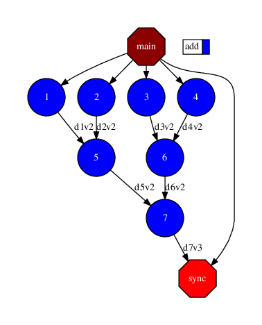
Figure 3 The dependency graph of the addition application
COMPSs has detected that the addition of a+b and c+d is independent,
and consequently, that they can be done in parallel. While the addition
of res1+res2 waits for the previous additions.
Check the performance
Let’s run it again with the tracing flag enabled:
$ runcompss-taddition.R
[ INFO] Inferred PYTHON language [ INFO] Using default location for project file: /opt/COMPSs//Runtime/configuration/xml/projects/default_project.xml [ INFO] Using default location for resources file: /opt/COMPSs//Runtime/configuration/xml/resources/default_resources.xml [ INFO] Using default execution type: compss ----------------- Executing addition.R -------------------------- Welcome to Extrae 3.8.3 [... Extrae prolog ...] WARNING: COMPSs Properties file is null. Setting default values [(843) API] - Starting COMPSs Runtime v3.4 The result is: 44 [... Extrae eplilog ...] mpi2prv: Congratulations! ./trace/addition.R_compss_trace.prv has been generated. [(24117) API] - Execution Finished ------------------------------------------------------------
The execution has finished successfully and the trace has been generated
in the $HOME/.COMPSs/<APP_NAME>_<00-99>/trace directory in prv format,
which can be displayed and analyzed with PARAVER.
Once Paraver has started, lets visualize the tasks:
Click in File and then in LoadConfiguration
Look for $COMPSS_HOME/Dependencies/paraver/cfgs/compss_tasks.cfg and click Open.
Note
In the case of using the PyCOMPSs CLI, the configuration files can be
obtained by downloading them from the COMPSs repository.
And you should see:
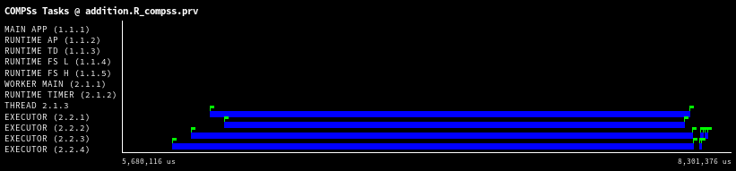
Figure 4 Trace of the addition.R application
The X axis represents the time, and the Y axis the deployed processes
(the first five (1.1.1-1.1.5) belong to the master and the next three belongs
to the master process in the worker (2.1.1-2.1.3) whose events are
shown with the compss_runtime.cfg configuration file).
The addition tasks are depicted in blue.
We can quickly see that the first four add tasks have been executed in parallel
(one per core), the next two as well, and finally, the last one that accumulates
all partial results at the end.
Paraver is a very powerful tool for performance analysis. For more information,
check the 🎯 Tracing Section.
Note
If you are using the COMPSs CLI, it is time to stop the COMPSs environment: