1.14. Machine Learning with dislib
This tutorial will show the different algorithms available in dislib.
Setup
First, we need to start an interactive PyCOMPSs session:
[1]:
import pycompss.interactive as ipycompss
import os
if 'BINDER_SERVICE_HOST' in os.environ:
    ipycompss.start(graph=True,
                    project_xml='../xml/project.xml',
                    resources_xml='../xml/resources.xml')
else:
    ipycompss.start(graph=True, monitor=1000)
********************************************************
**************** PyCOMPSs Interactive ******************
********************************************************
*          .-~~-.--.           ______        ______    *
*         :         )         |____  \      /  __  \   *
*   .~ ~ -.\       /.- ~~ .      __) |      | |  | |   *
*   >       `.   .'       <     |__  |      | |  | |   *
*  (         .- -.         )   ____) |   _  | |__| |   *
*   `- -.-~  `- -'  ~-.- -'   |______/  |_| \______/   *
*     (        :        )           _ _ .-:            *
*      ~--.    :    .--~        .-~  .-~  }            *
*          ~-.-^-.-~ \_      .~  .-~   .~              *
*                   \ \ '     \ '_ _ -~                *
*                    \`.\`.    //                      *
*           . - ~ ~-.__\`.\`-.//                       *
*       .-~   . - ~  }~ ~ ~-.~-.                       *
*     .' .-~      .-~       :/~-.~-./:                 *
*    /_~_ _ . - ~                 ~-.~-._              *
*                                     ~-.<             *
********************************************************
* - Starting COMPSs runtime...                         *
* - Log path : /home/user/.COMPSs/Interactive_14/
* - PyCOMPSs Runtime started... Have fun!              *
********************************************************
Next, we import dislib and we are all set to start working!
[2]:
import dislib as ds
Load the MNIST dataset
[3]:
x, y = ds.load_svmlight_file('/tmp/mnist/mnist', # Download the dataset
                             block_size=(10000, 784), n_features=784, store_sparse=False)
[4]:
x.shape
[4]:
(60000, 784)
[5]:
y.shape
[5]:
(60000, 1)
[6]:
y_array = y.collect()
y_array
[6]:
array([5., 0., 4., ..., 5., 6., 8.])
[7]:
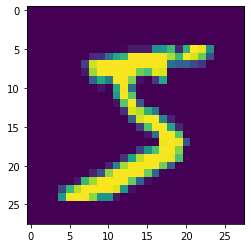
img = x[0].collect().reshape(28,28)
[8]:
%matplotlib inline
import matplotlib.pyplot as plt
plt.imshow(img)
[8]:
<matplotlib.image.AxesImage at 0x7f6fe8427be0>
[9]:
int(y[0].collect())
[9]:
5
dislib algorithms
Preprocessing
[10]:
from dislib.preprocessing import StandardScaler
from dislib.decomposition import PCA
Clustering
[11]:
from dislib.cluster import KMeans
from dislib.cluster import DBSCAN
from dislib.cluster import GaussianMixture
Classification
[12]:
from dislib.classification import CascadeSVM
from dislib.classification import RandomForestClassifier
Recommendation
[13]:
from dislib.recommendation import ALS
Model selection
[14]:
from dislib.model_selection import GridSearchCV
Others
[15]:
from dislib.regression import LinearRegression
from dislib.neighbors import NearestNeighbors
/home/user/github/dislib/dislib/regression/lasso/base.py:20: UserWarning: Cannot import cvxpy module. Lasso estimator will not work.
  warnings.warn('Cannot import cvxpy module. Lasso estimator will not work.')
/home/user/github/dislib/dislib/optimization/admm/base.py:16: UserWarning: Cannot import cvxpy module. ADMM estimator will not work.
  warnings.warn('Cannot import cvxpy module. ADMM estimator will not work.')
Examples
KMeans
[16]:
kmeans = KMeans(n_clusters=10)
pred_clusters = kmeans.fit_predict(x).collect()
Get the number of images of each class in the cluster 0:
[17]:
from collections import Counter
Counter(y_array[pred_clusters==0])
[17]:
Counter({7.0: 3173,
         2.0: 76,
         9.0: 732,
         3.0: 22,
         8.0: 42,
         4.0: 70,
         1.0: 5,
         5.0: 7,
         6.0: 1})
GaussianMixture
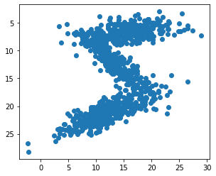
Fit the GaussianMixture with the painted pixels of a single image:
[18]:
import numpy as np
img_filtered_pixels = np.stack([np.array([i, j]) for i in range(28) for j in range(28) if img[i,j] > 10])
img_pixels = ds.array(img_filtered_pixels, block_size=(50,2))
gm = GaussianMixture(n_components=7, random_state=0)
gm.fit(img_pixels)
Get the parameters that define the Gaussian components:
[19]:
from pycompss.api.api import compss_wait_on
means = compss_wait_on(gm.means_)
covariances = compss_wait_on(gm.covariances_)
weights = compss_wait_on(gm.weights_)
Use the Gaussian mixture model to sample random pixels replicating the original distribution:
[20]:
samples = np.concatenate([np.random.multivariate_normal(means[i], covariances[i], int(weights[i]*1000))
                    for i in range(7)])
plt.scatter(samples[:,1], samples[:,0])
plt.gca().set_aspect('equal', adjustable='box')
plt.gca().invert_yaxis()
plt.draw()
PCA
[21]:
pca = PCA()
pca.fit(x)
[21]:
PCA()
Calculate the explained variance of the 10 first eigenvectors:
[22]:
explained_variance = pca.explained_variance_.collect()
sum(explained_variance[0:10])/sum(explained_variance)
[22]:
0.4881498035493399
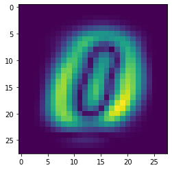
Show the weights of the first eigenvector:
[23]:
plt.imshow(np.abs(pca.components_.collect()[0]).reshape(28,28))
[23]:
<matplotlib.image.AxesImage at 0x7f6fd89aa2e0>
RandomForestClassifier
[24]:
rf = RandomForestClassifier(n_estimators=5, max_depth=3)
rf.fit(x, y)
[24]:
RandomForestClassifier(max_depth=3, n_estimators=5)
Use the test dataset to get an accuracy score:
[25]:
x_test, y_test = ds.load_svmlight_file('/tmp/mnist/mnist.test', block_size=(10000, 784), n_features=784, store_sparse=False)
score = rf.score(x_test, y_test)
print(compss_wait_on(score))
0.6132
Close the session
To finish the session, we need to stop PyCOMPSs:
[26]:
ipycompss.stop()
********************************************************
*************** STOPPING PyCOMPSs ******************
********************************************************
Checking if any issue happened.
Warning: some of the variables used with PyCOMPSs may
         have not been brought to the master.
********************************************************